
Bifurcation Analysis of the Keynesian Cross Model: Method and G is constant
:::info
Xinyu Li, University of Washington.
:::
Table of Links
Abstract and Introduction
2. Method and 2.1. G is constant
2.2. Linear Relation between G and I
2.3. Nonlinear Quadratic Relation between G and I
3. Results
4. Conclusion and References
2. Method
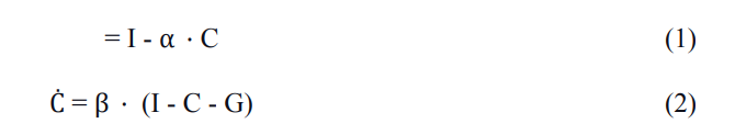
The Keynesian cross model builds upon two ordinary differential equations [6]:
\
\
where C ≥ 0 is the rate of consumer spending, I ≥ 0 is the national income, and G ≥ 0 is the rate of government spending. The parameters α and β satisfy 1 < α < ∞, 1 ≤ β < ∞. Three relations between government spending and national income are discussed in the following subsections.
2.1. G is constant
Consider a model consisting of equations (1) and (2) along with a constant government spending G. To determine the equilibrium state for this model, I find the point where = Ċ = 0. Rearranging terms, I obtain the following equilibrium:
\
In order to calculate the stability of this fixed point, I compute the Jacobian matrix and eigenvalues:
\
\
:::info
This paper is available on arxiv under CC 4.0 license.
:::
\
Welcome to Billionaire Club Co LLC, your gateway to a brand-new social media experience! Sign up today and dive into over 10,000 fresh daily articles and videos curated just for your enjoyment. Enjoy the ad free experience, unlimited content interactions, and get that coveted blue check verification—all for just $1 a month!
Account Frozen
Your account is frozen. You can still view content but cannot interact with it.
Please go to your settings to update your account status.
Open Profile Settings